Unit 2, part 2 of the Deep Reinforcement Learning Class with Hugging Face 🤗

⚠️ A new updated version of this article is available here 👉 https://huggingface.co/deep-rl-course/unit1/introduction

This article is part of the Deep Reinforcement Learning Class. A free course from beginner to expert. Check the syllabus here.

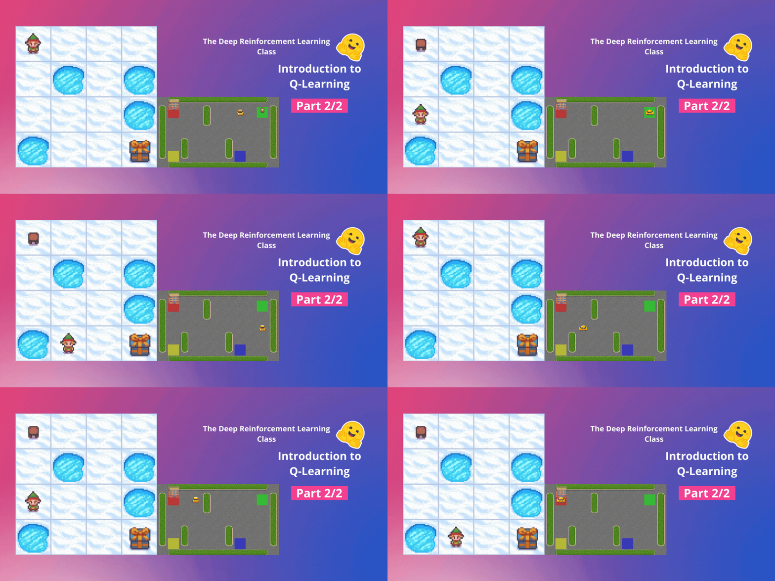
⚠️ A new updated version of this article is available here 👉 https://huggingface.co/deep-rl-course/unit1/introduction

This article is part of the Deep Reinforcement Learning Class. A free course from beginner to expert. Check the syllabus here.

In the first part of this unit, we learned about the value-based methods and the difference between Monte Carlo and Temporal Difference Learning.

So, in the second part, we’ll study Q-Learning, and implement our first RL agent from scratch, a Q-Learning agent, and will train it in two environments:

Frozen Lake v1 ❄️: where our agent will need to go from the starting state (S) to the goal state (G) by walking only on frozen tiles (F) and avoiding holes (H).
An autonomous taxi 🚕: where the agent will need to learn to navigate a city to transport its passengers from point A to point B.

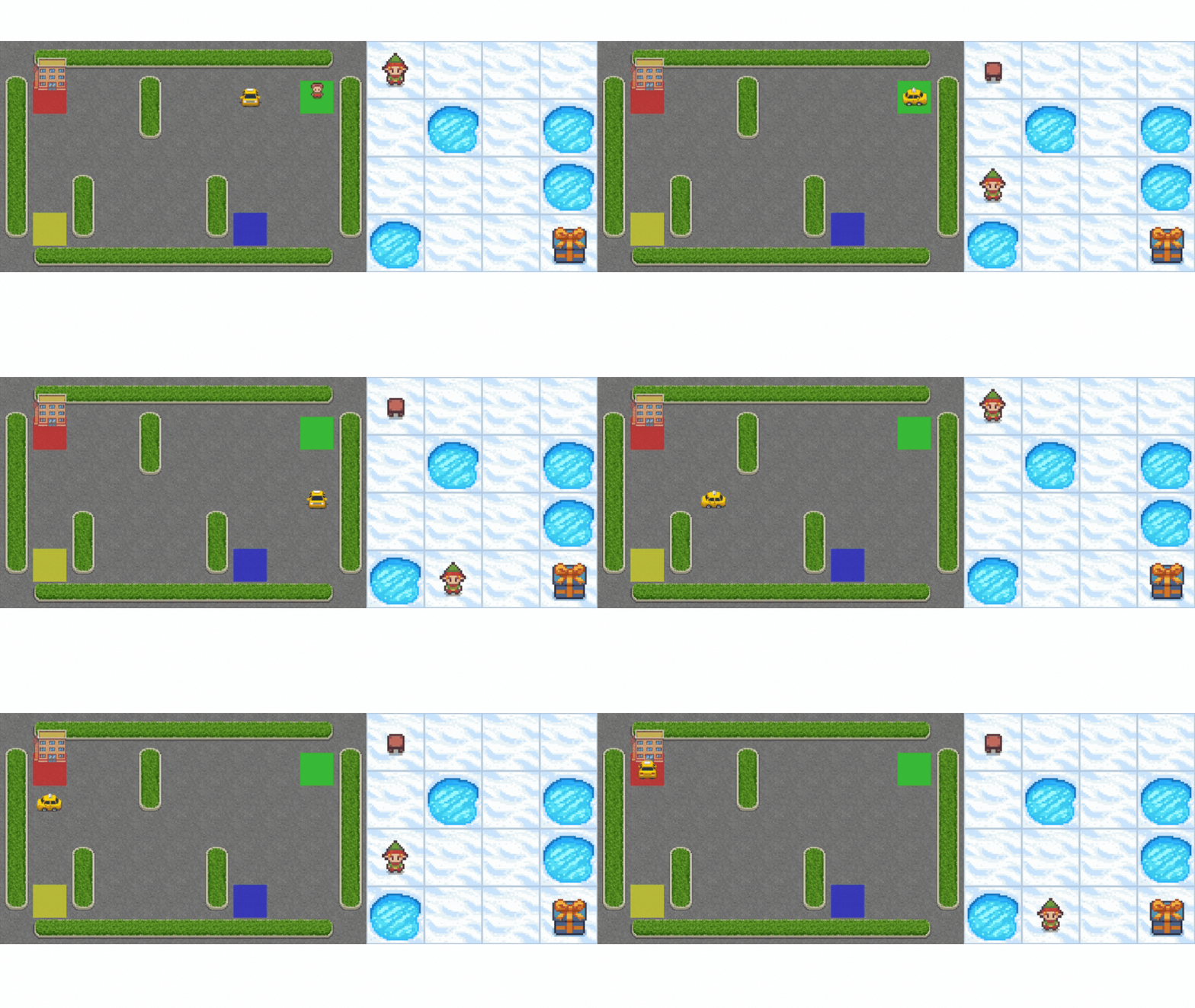
This unit is fundamental if you want to be able to work on Deep Q-Learning (Unit 3).

So let’s get started! 🚀

Introducing Q-Learning

What is Q-Learning?

Q-Learning is an off-policy value-based method that uses a TD approach to train its action-value function:

Off-policy: we'll talk about that at the end of this chapter.
Value-based method: finds the optimal policy indirectly by training a value or action-value function that will tell us the value of each state or each state-action pair.
Uses a TD approach: updates its action-value function at each step instead of at the end of the episode.

Q-Learning is the algorithm we use to train our Q-Function, an action-value function that determines the value of being at a particular state and taking a specific action at that state.

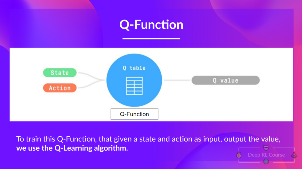
Given a state and action, our Q Function outputs a state-action value (also called Q-value)

The Q comes from "the Quality" of that action at that state.

Internally, our Q-function has a Q-table, a table where each cell corresponds to a state-action value pair value. Think of this Q-table as the memory or cheat sheet of our Q-function.

If we take this maze example:

The Q-Table is initialized. That's why all values are = 0. This table contains, for each state, the four state-action values.

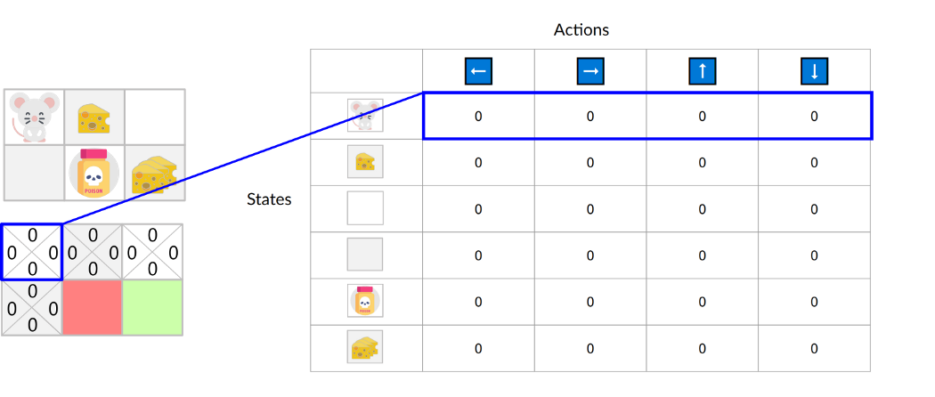
Here we see that the state-action value of the initial state and going up is 0:

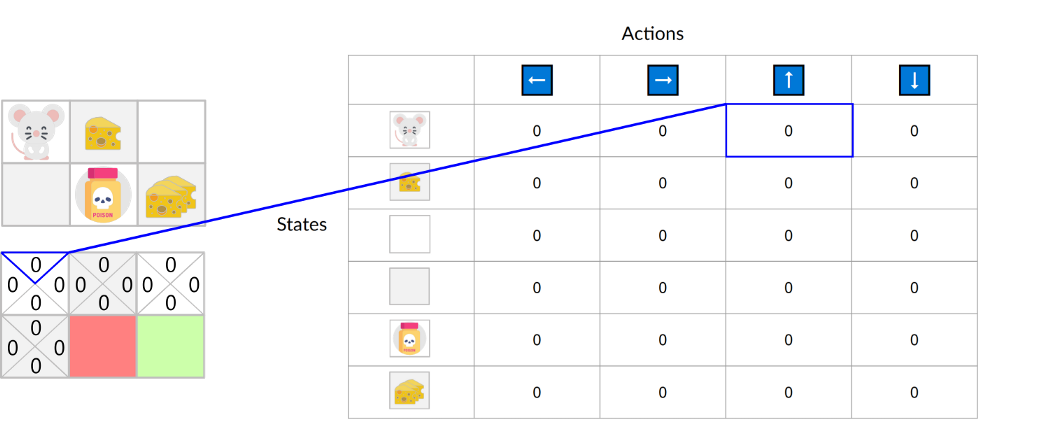
Therefore, Q-function contains a Q-table that has the value of each-state action pair. And given a state and action, our Q-Function will search inside its Q-table to output the value.

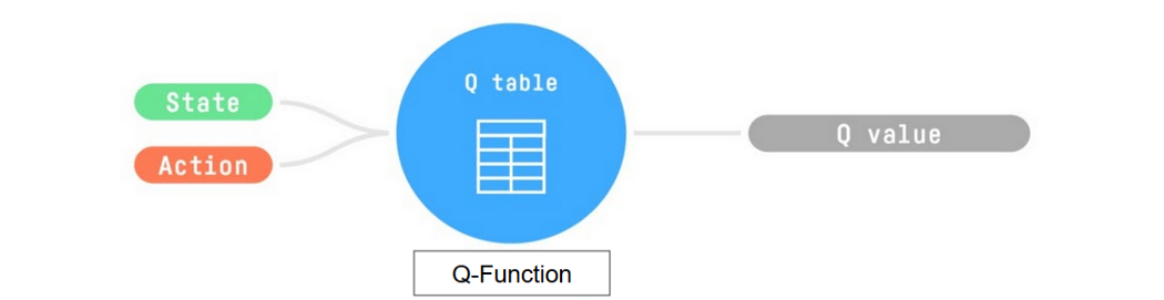
Given a state and action pair, our Q-function will search inside its Q-table to output the state-action pair value (the Q value).

If we recap, Q-Learning is the RL algorithm that:

Trains Q-Function (an action-value function) which internally is a Q-table that contains all the state-action pair values.
Given a state and action, our Q-Function will search into its Q-table the corresponding value.
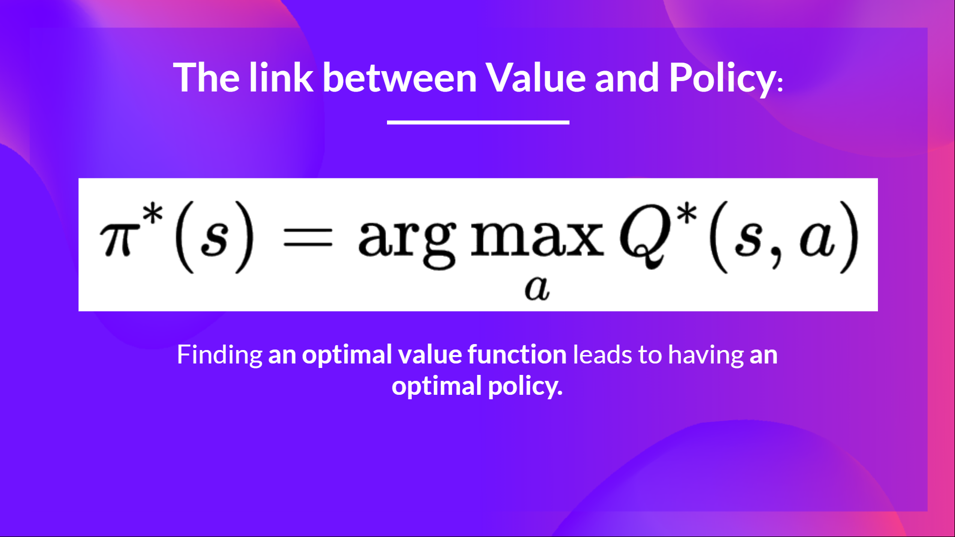
When the training is done, we have an optimal Q-function, which means we have optimal Q-Table.
And if we have an optimal Q-function, we have an optimal policy since we know for each state what is the best action to take.

But, in the beginning, our Q-Table is useless since it gives arbitrary values for each state-action pair (most of the time, we initialize the Q-Table to 0 values). But, as we'll explore the environment and update our Q-Table, it will give us better and better approximations.

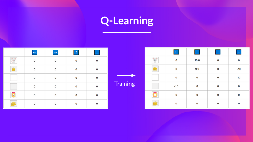
We see here that with the training, our Q-Table is better since, thanks to it, we can know the value of each state-action pair.

So now that we understand what Q-Learning, Q-Function, and Q-Table are, let's dive deeper into the Q-Learning algorithm.

The Q-Learning algorithm

This is the Q-Learning pseudocode; let's study each part and see how it works with a simple example before implementing it. Don't be intimidated by it, it's simpler than it looks! We'll go over each step.

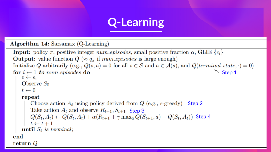
Step 1: We initialize the Q-Table

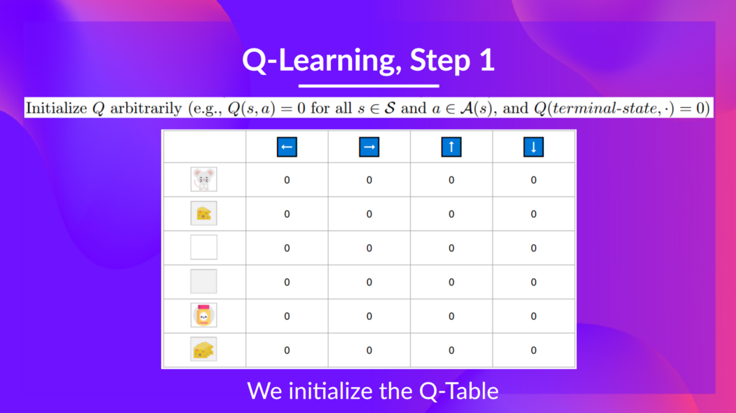
We need to initialize the Q-Table for each state-action pair. Most of the time, we initialize with values of 0.

Step 2: Choose action using Epsilon Greedy Strategy

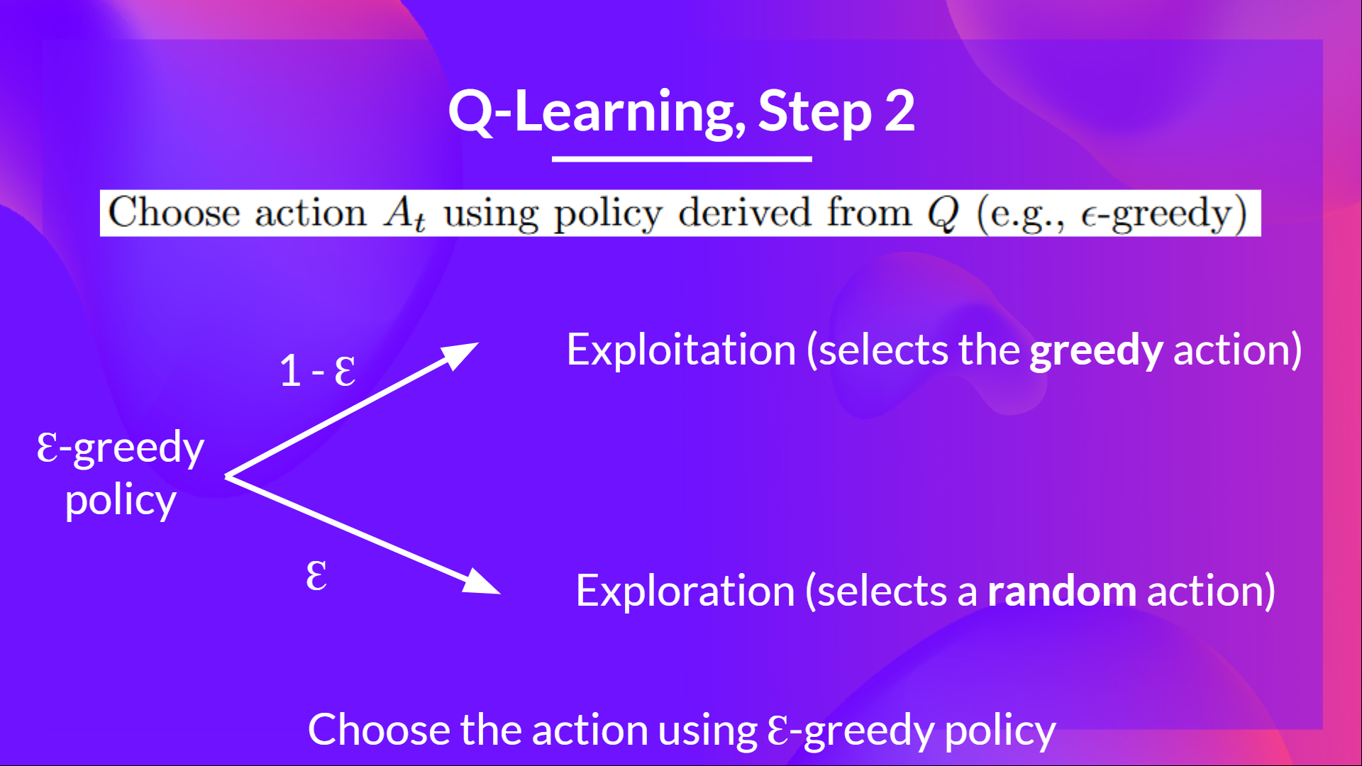
Epsilon Greedy Strategy is a policy that handles the exploration/exploitation trade-off.

The idea is that we define epsilon ɛ = 1.0:

With probability 1 — ɛ : we do exploitation (aka our agent selects the action with the highest state-action pair value).
With probability ɛ: we do exploration (trying random action).

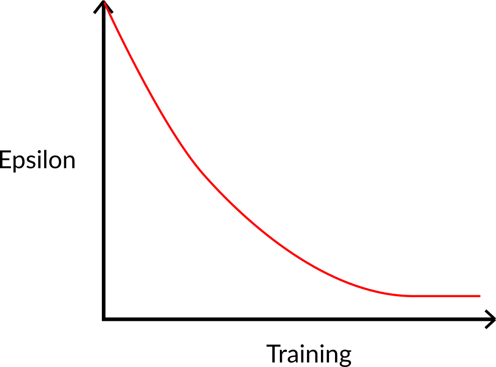
At the beginning of the training, the probability of doing exploration will be huge since ɛ is very high, so most of the time, we'll explore. But as the training goes on, and consequently our Q-Table gets better and better in its estimations, we progressively reduce the epsilon value since we will need less and less exploration and more exploitation.

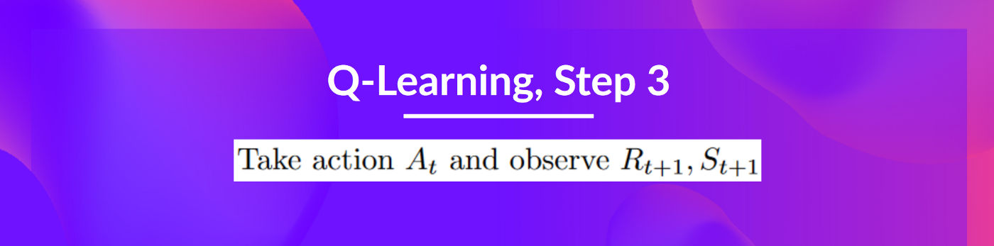
Step 3: Perform action At, gets reward Rt+1 and next state St+1

Step 4: Update Q(St, At)

Remember that in TD Learning, we update our policy or value function (depending on the RL method we choose) after one step of the interaction.

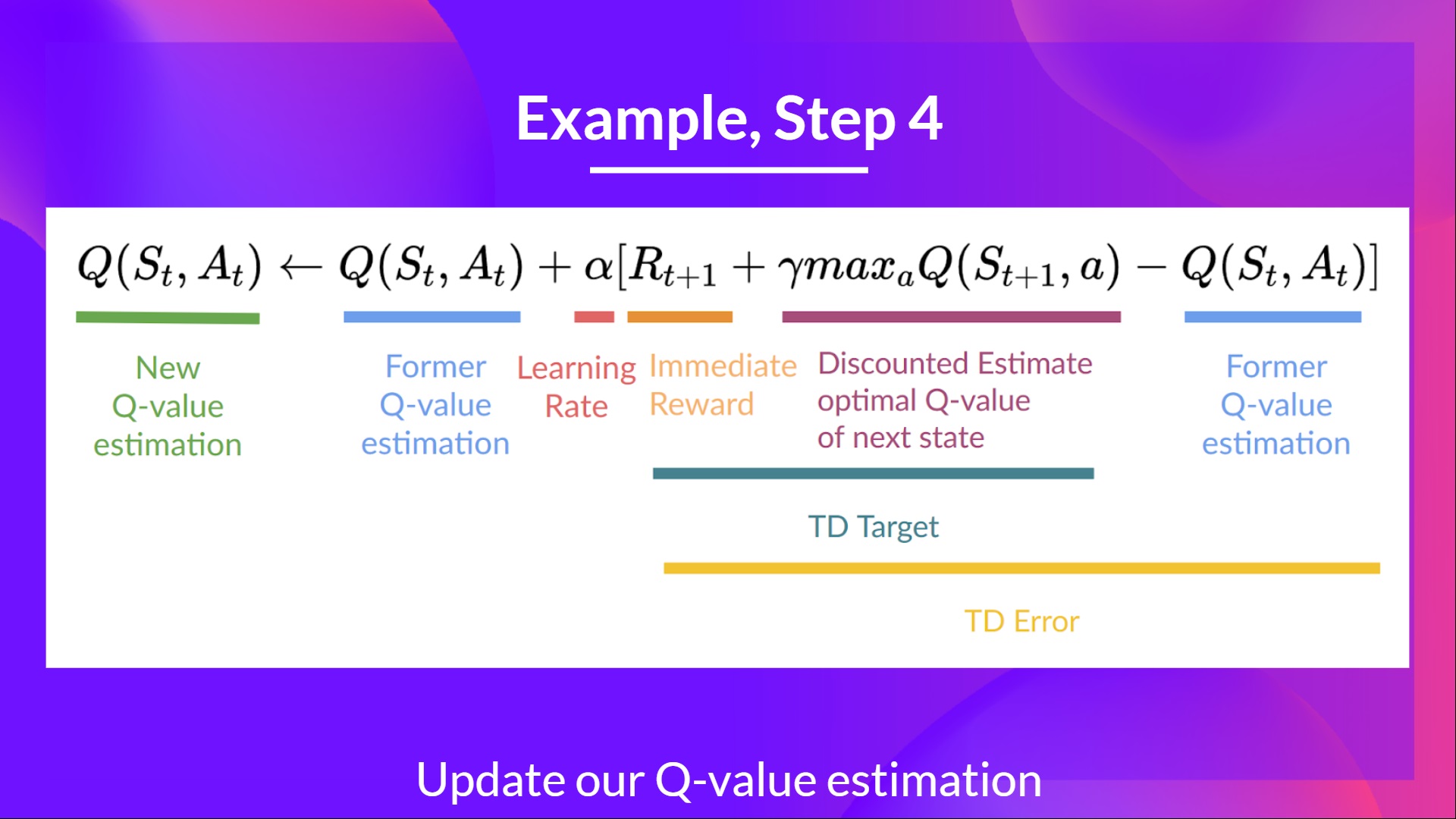
To produce our TD target, we used the immediate reward Rt+1R_{t+1} plus the discounted value of the next state best state-action pair (we call that bootstrap).

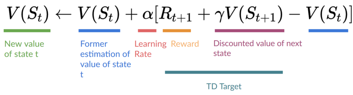
Therefore, our Q(St,At)Q(S_t, A_t) update formula goes like this:

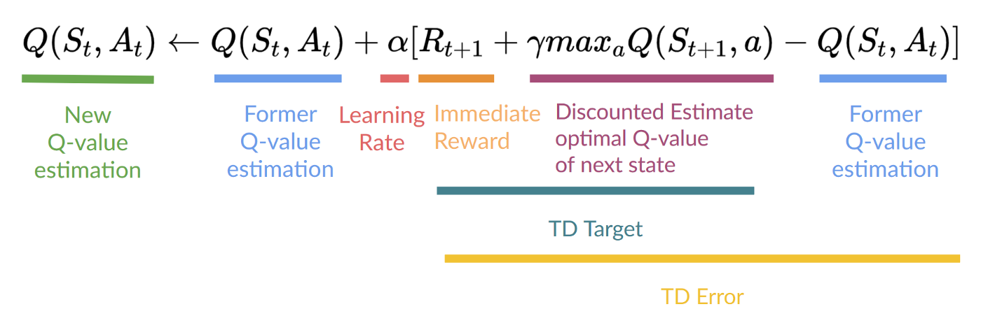
It means that to update our Q(St,At)Q(S_t, A_t):

We need St,At,Rt+1,St+1S_t, A_t, R_{t+1}, S_{t+1}.
To update our Q-value at a given state-action pair, we use the TD target.

How do we form the TD target?

We obtain the reward after taking the action Rt+1R_{t+1}.
To get the best next-state-action pair value, we use a greedy policy to select the next best action. Note that this is not an epsilon greedy policy, this will always take the action with the highest state-action value.

Then when the update of this Q-value is done. We start in a new_state and select our action using our epsilon-greedy policy again.

It's why we say that this is an off-policy algorithm.

Off-policy vs On-policy

The difference is subtle:

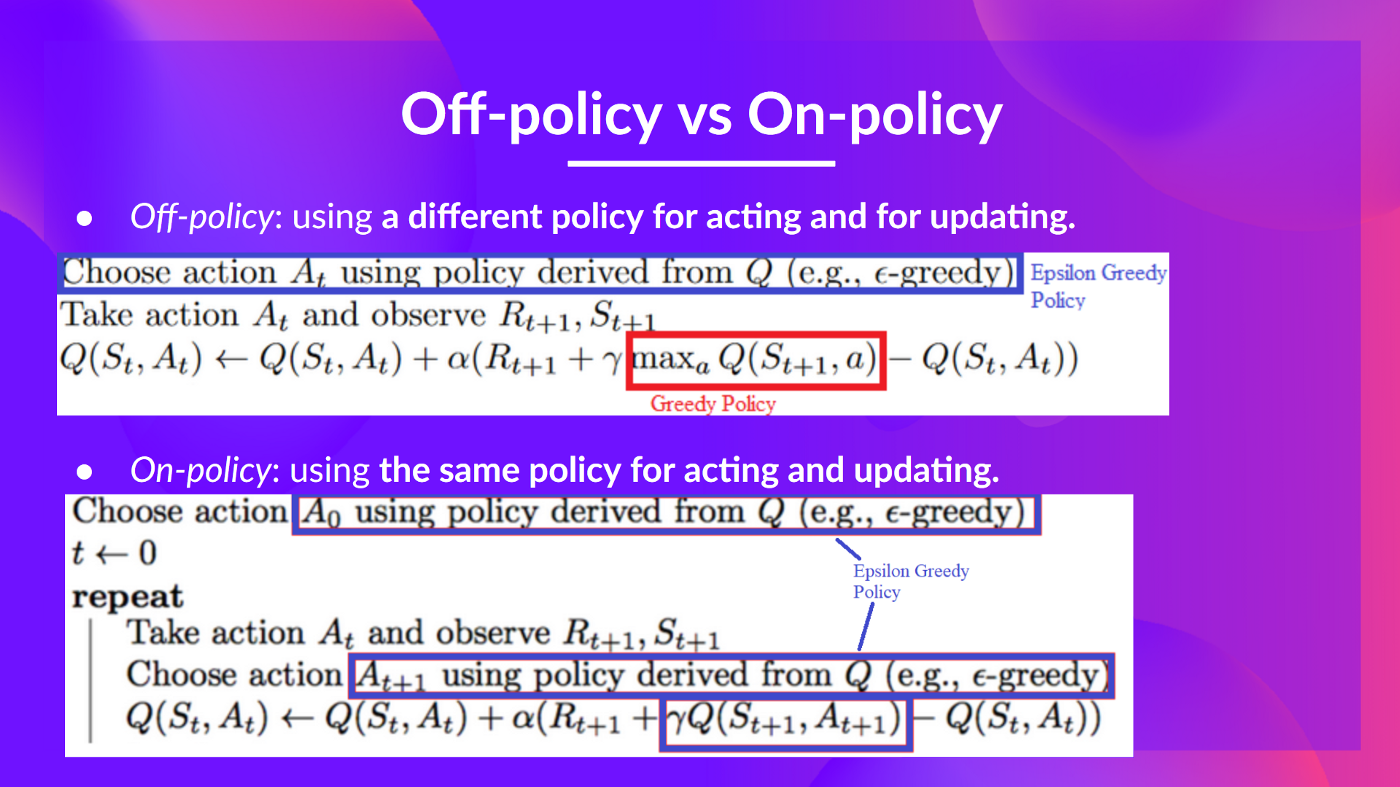
Off-policy: using a different policy for acting and updating.

For instance, with Q-Learning, the Epsilon greedy policy (acting policy), is different from the greedy policy that is used to select the best next-state action value to update our Q-value (updating policy).

Acting Policy

Is different from the policy we use during the training part:

Updating policy

On-policy: using the same policy for acting and updating.

For instance, with Sarsa, another value-based algorithm, the Epsilon-Greedy Policy selects the next_state-action pair, not a greedy policy.

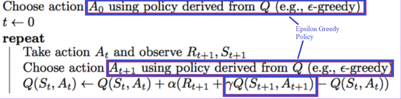
Sarsa

A Q-Learning example

To better understand Q-Learning, let's take a simple example:

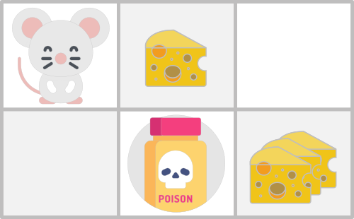
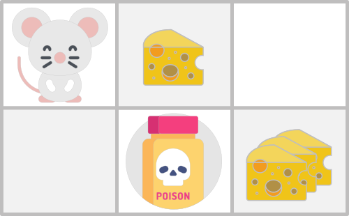
You're a mouse in this tiny maze. You always start at the same starting point.
The goal is to eat the big pile of cheese at the bottom right-hand corner and avoid the poison. After all, who doesn't like cheese?
The episode ends if we eat the poison, eat the big pile of cheese or if we spent more than five steps.
The learning rate is 0.1
The gamma (discount rate) is 0.99

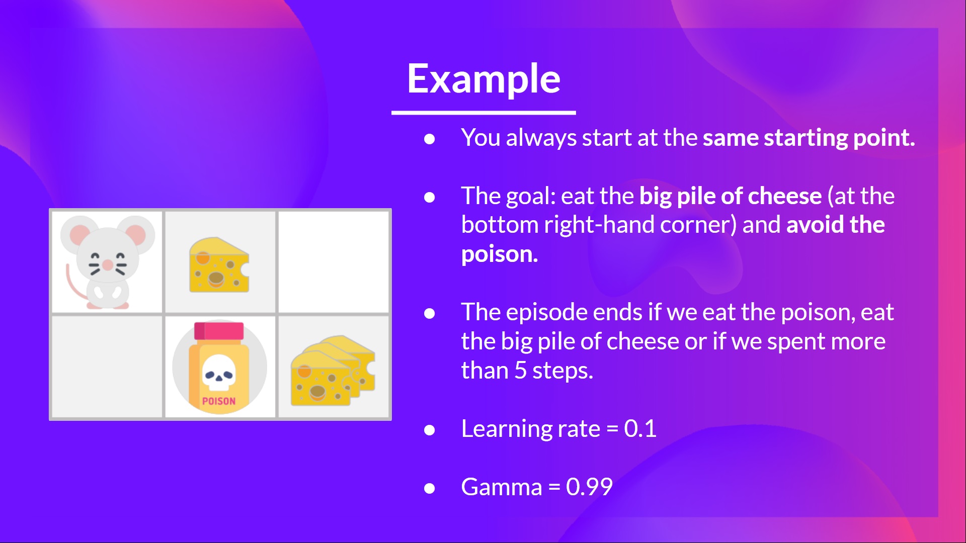
The reward function goes like this:

+0: Going to a state with no cheese in it.
+1: Going to a state with a small cheese in it.
+10: Going to the state with the big pile of cheese.
-10: Going to the state with the poison and thus die.
+0 If we spend more than five steps.

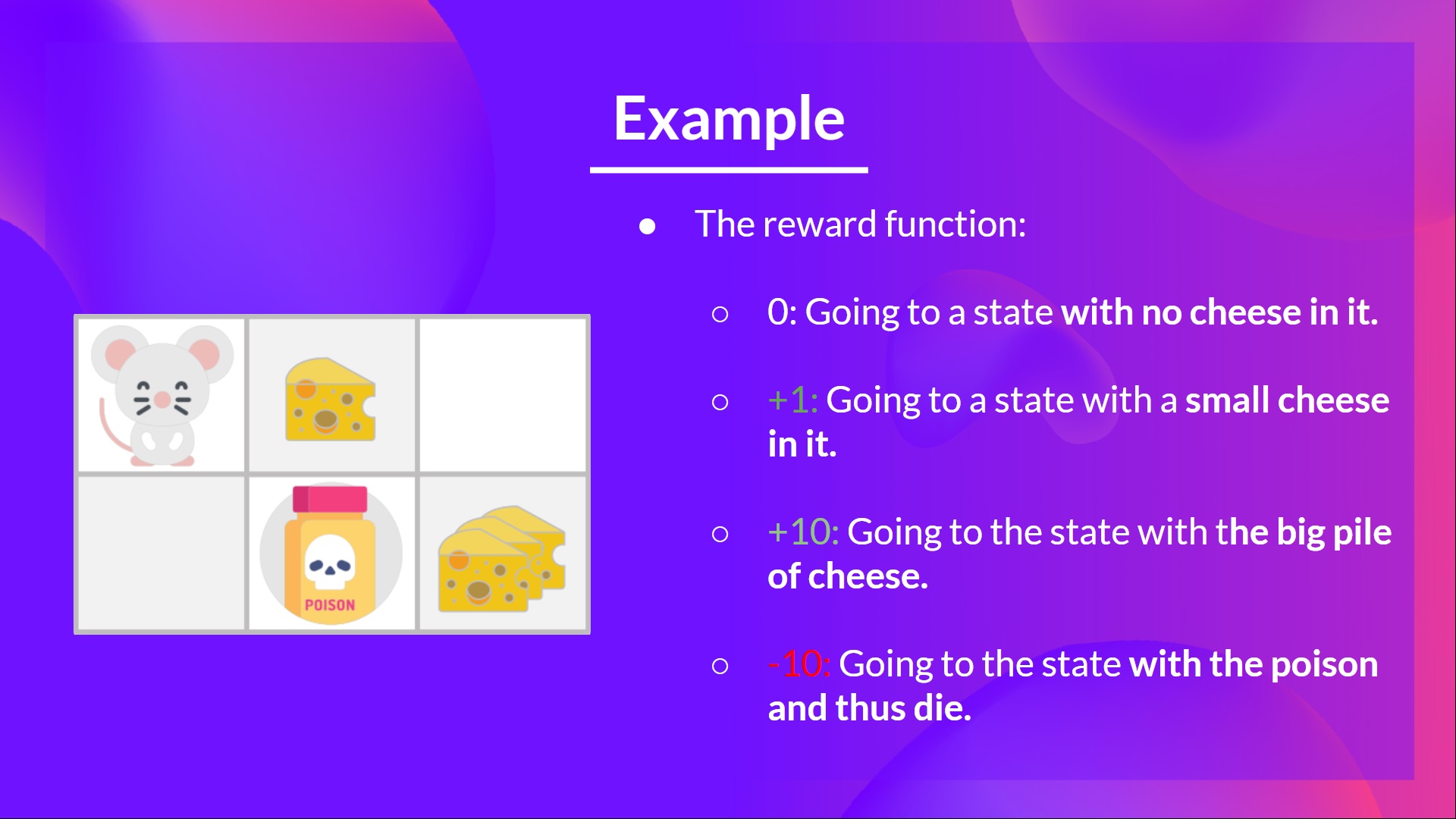
To train our agent to have an optimal policy (so a policy that goes right, right, down), we will use the Q-Learning algorithm.

Step 1: We initialize the Q-Table

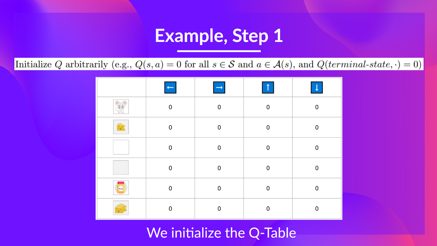
So, for now, our Q-Table is useless; we need to train our Q-function using the Q-Learning algorithm.

Let's do it for 2 training timesteps:

Training timestep 1:

Step 2: Choose action using Epsilon Greedy Strategy

Because epsilon is big = 1.0, I take a random action, in this case, I go right.

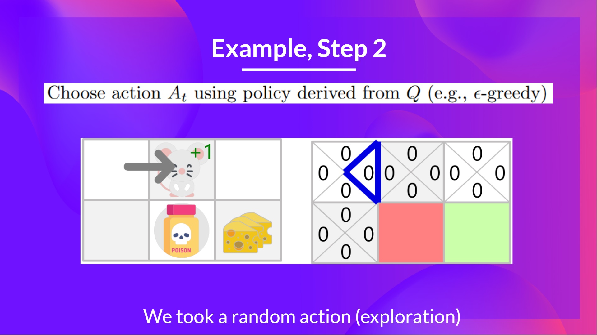
Step 3: Perform action At, gets Rt+1 and St+1

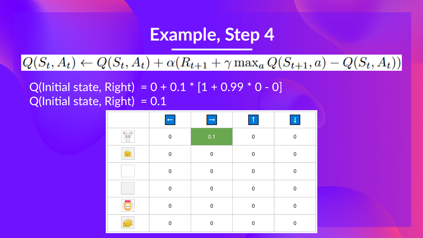
By going right, I've got a small cheese, so Rt+1=1R_{t+1} = 1, and I'm in a new state.

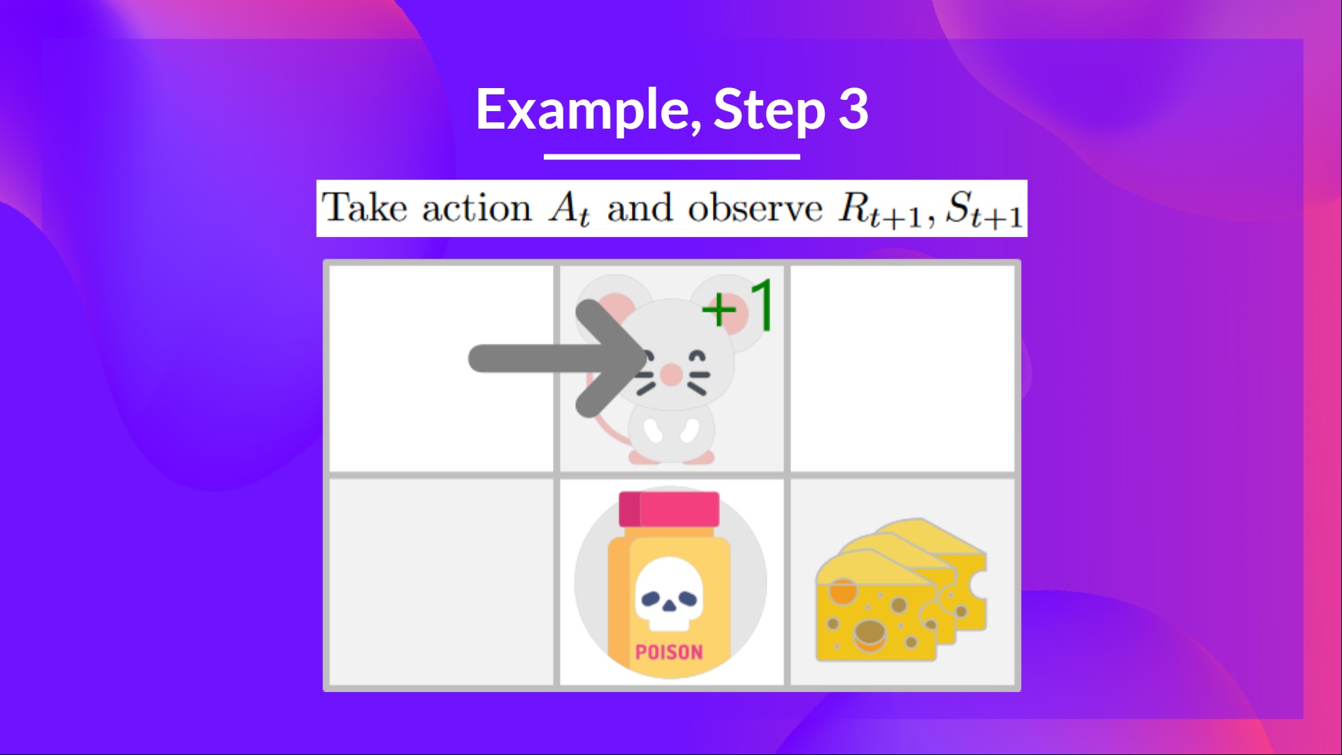
Step 4: Update Q(St,At)Q(S_t, A_t)

We can now update Q(St,At)Q(S_t, A_t) using our formula.

Training timestep 2:

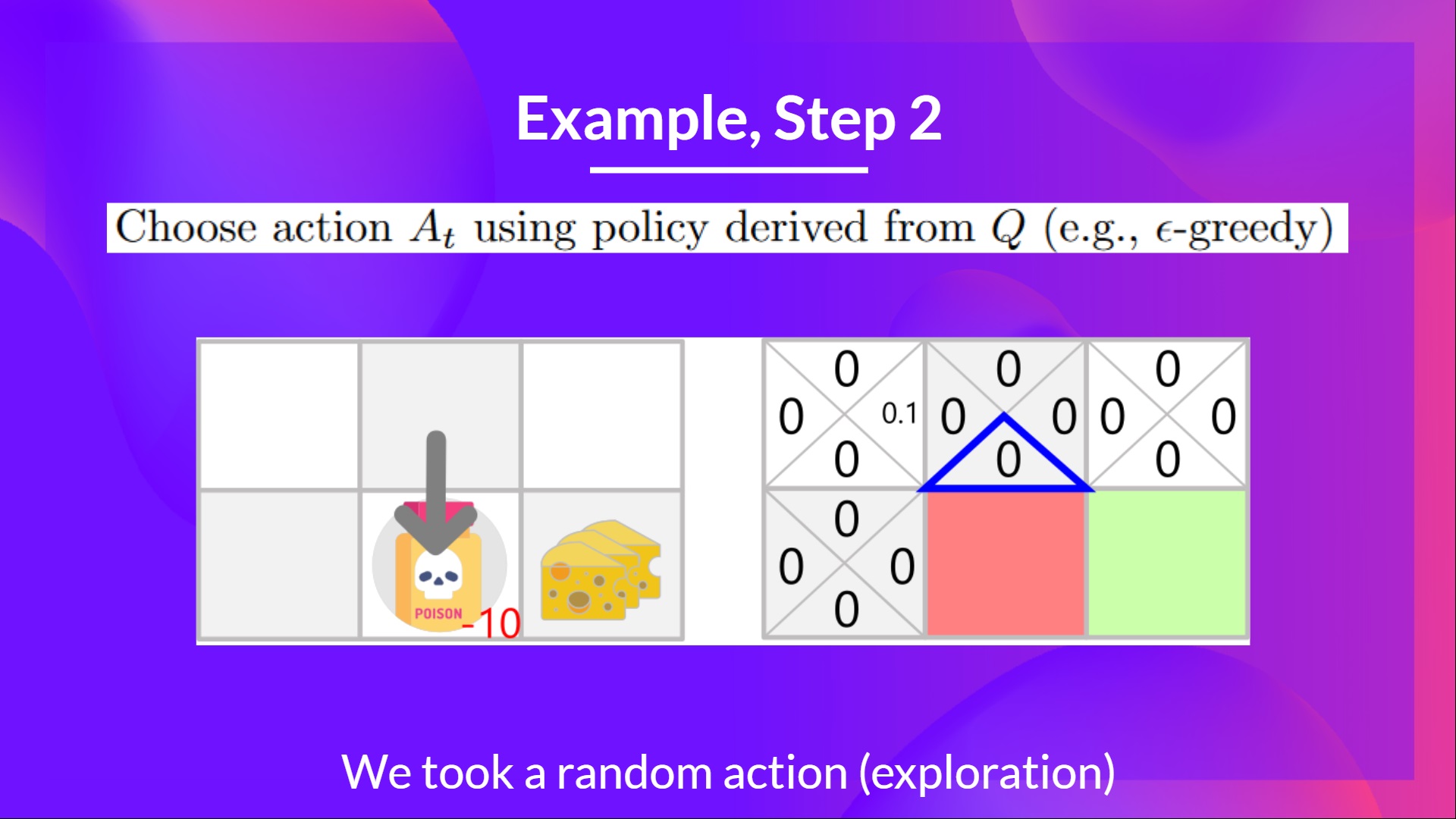
Step 2: Choose action using Epsilon Greedy Strategy

I take a random action again, since epsilon is big 0.99 (since we decay it a little bit because as the training progress, we want less and less exploration).

I took action down. Not a good action since it leads me to the poison.

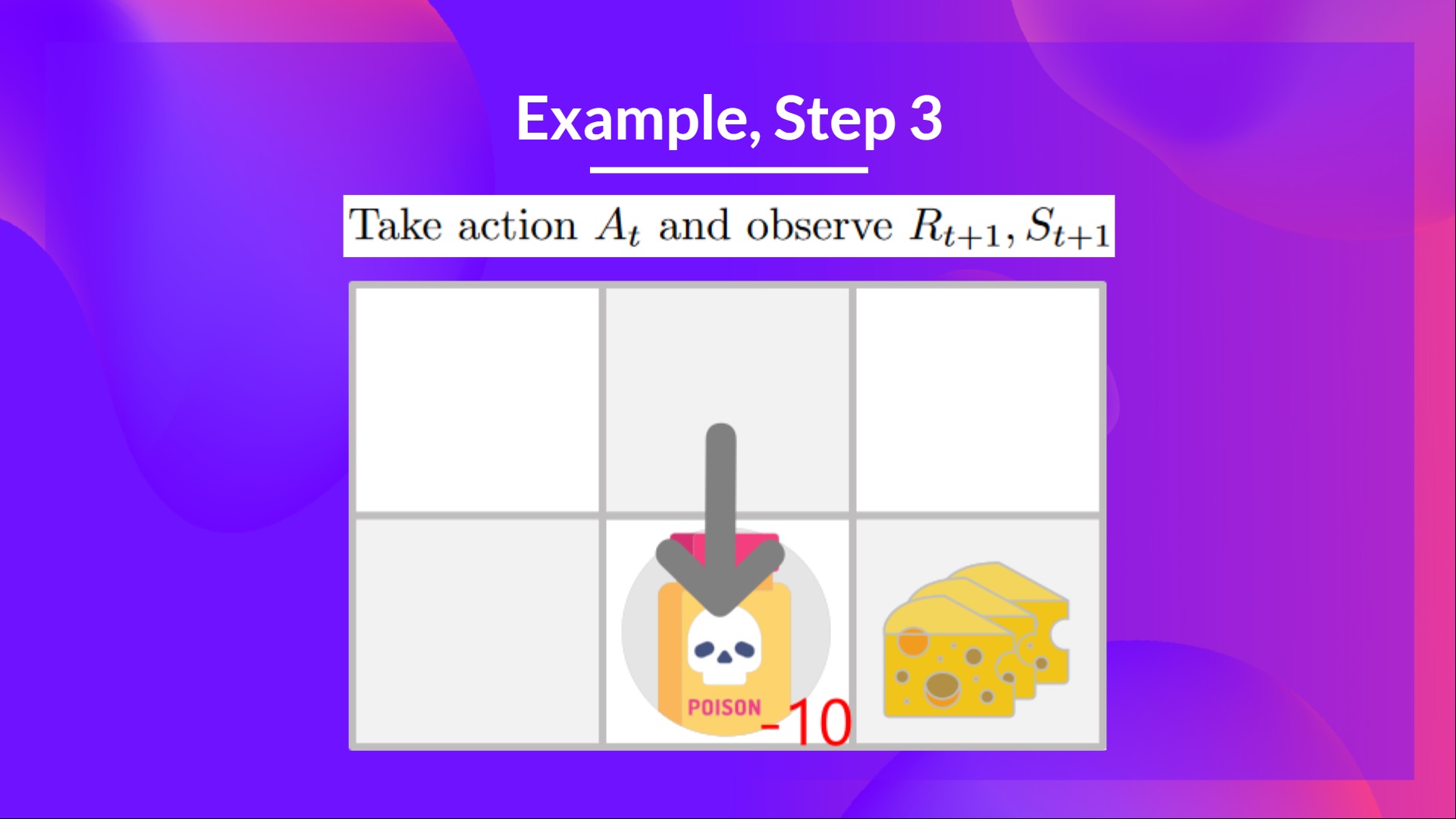
Step 3: Perform action At, gets Rt+1R_{t+1} and St+1

Because I go to the poison state, I get Rt+1=−10R_{t+1} = -10, and I die.

Step 4: Update Q(St,At)Q(S_t, A_t)

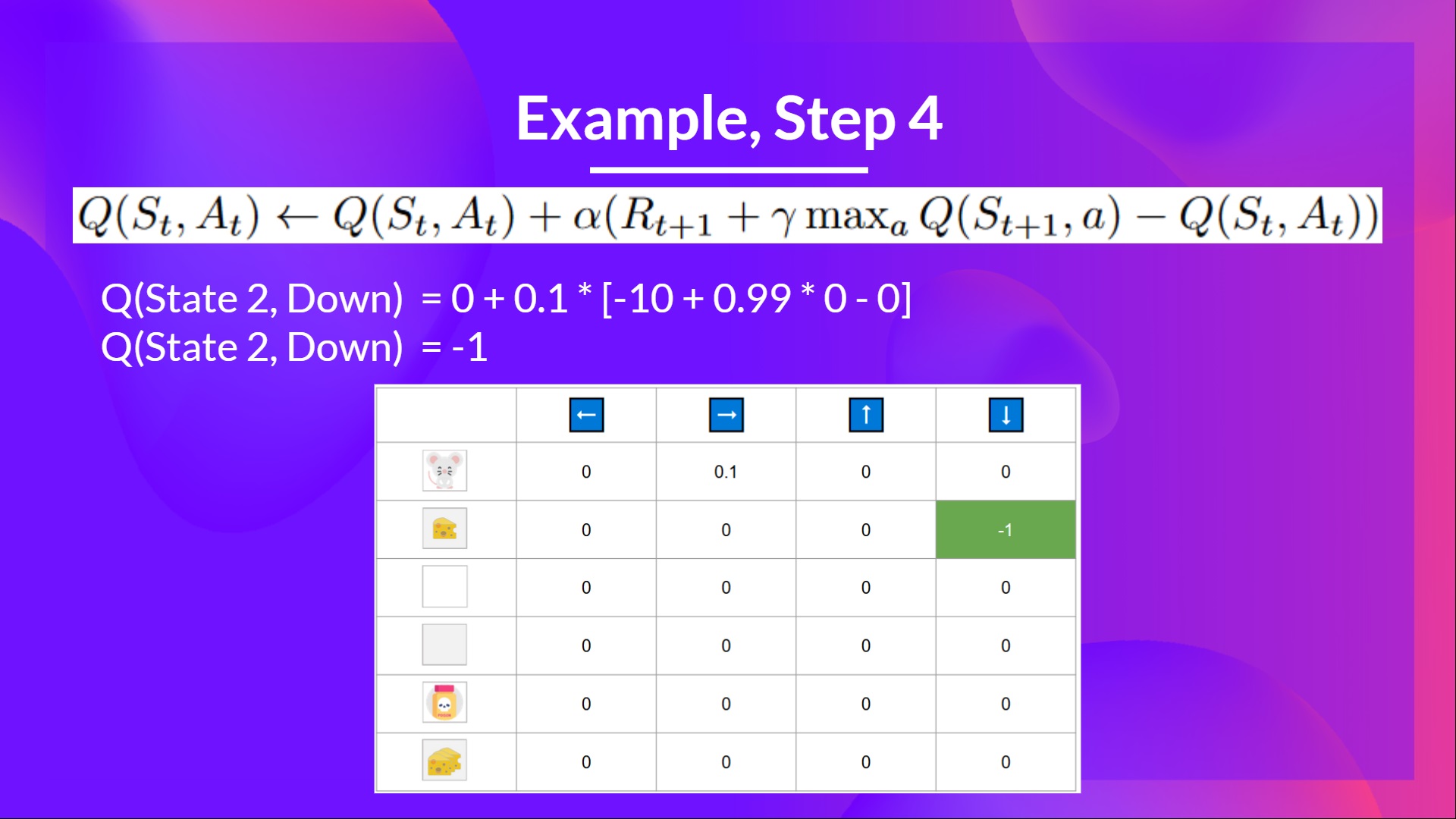
Because we're dead, we start a new episode. But what we see here is that with two explorations steps, my agent became smarter.

As we continue exploring and exploiting the environment and updating Q-values using TD target, Q-Table will give us better and better approximations. And thus, at the end of the training, we'll get an estimate of the optimal Q-Function.

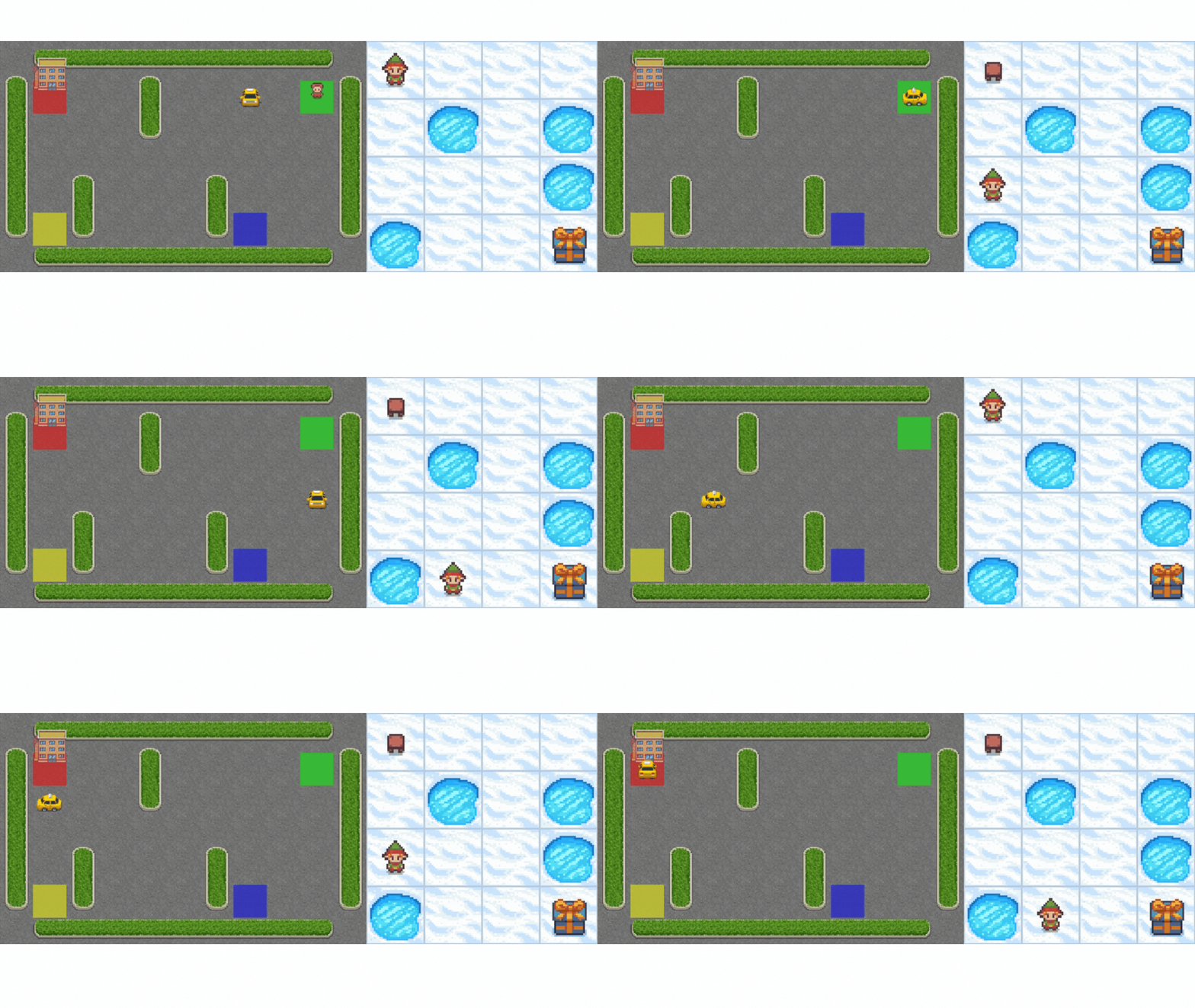
Now that we studied the theory of Q-Learning, let's implement it from scratch. A Q-Learning agent that we will train in two environments:

Frozen-Lake-v1 ❄️ (non-slippery version): where our agent will need to go from the starting state (S) to the goal state (G) by walking only on frozen tiles (F) and avoiding holes (H).
An autonomous taxi 🚕 will need to learn to navigate a city to transport its passengers from point A to point B.

Start the tutorial here 👉 https://colab.research.google.com/github/huggingface/deep-rl-class/blob/main/unit2/unit2.ipynb

The leaderboard 👉 https://huggingface.co/spaces/chrisjay/Deep-Reinforcement-Learning-Leaderboard

Congrats on finishing this chapter! There was a lot of information. And congrats on finishing the tutorials. You’ve just implemented your first RL agent from scratch and shared it on the Hub 🥳.

Implementing from scratch when you study a new architecture is important to understand how it works.

That’s normal if you still feel confused with all these elements. This was the same for me and for all people who studied RL.

Take time to really grasp the material before continuing.

And since the best way to learn and avoid the illusion of competence is to test yourself. We wrote a quiz to help you find where you need to reinforce your study. Check your knowledge here 👉 https://github.com/huggingface/deep-rl-class/blob/main/unit2/quiz2.md

It’s essential to master these elements and having a solid foundations before entering the fun part. Don't hesitate to modify the implementation, try ways to improve it and change environments, the best way to learn is to try things on your own!

We published additional readings in the syllabus if you want to go deeper 👉 https://github.com/huggingface/deep-rl-class/blob/main/unit2/README.md

In the next unit, we’re going to learn about Deep-Q-Learning.

And don't forget to share with your friends who want to learn 🤗 !

Finally, we want to improve and update the course iteratively with your feedback. If you have some, please fill this form 👉 https://forms.gle/3HgA7bEHwAmmLfwh9

An Introduction to Q-Learning Part 2/2

Unit 2, part 2 of the Deep Reinforcement Learning Class with Hugging Face 🤗

Introducing Q-Learning

What is Q-Learning?

The Q-Learning algorithm

Off-policy vs On-policy

A Q-Learning example

Keep learning, stay awesome,